understanding LLM decoding strategies

12 Jun, 2026

so, while working on a personal project of running an SLM on Apple silicon, I came across the phenomenon of decoding in LLMs. While I had read of an overview of what the different strategies do, I had never gone into the mathematics of it all. So this post does exactly that.

Let’s start off with what decoding actually is, and its several basic techniques…

1. Greedy Decoding:
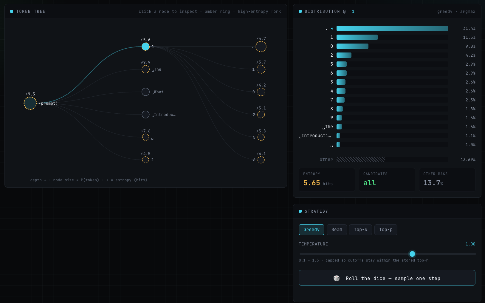
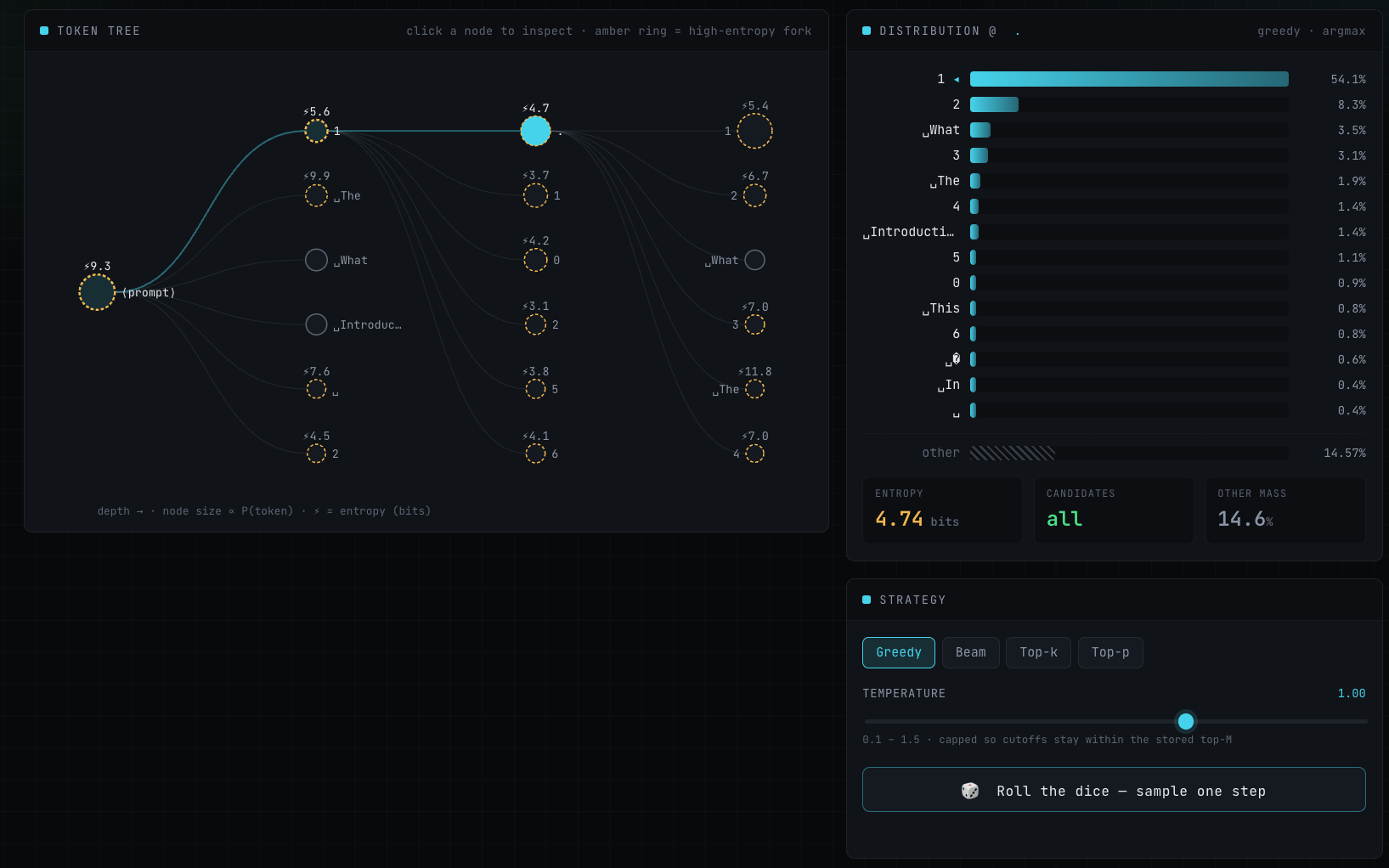
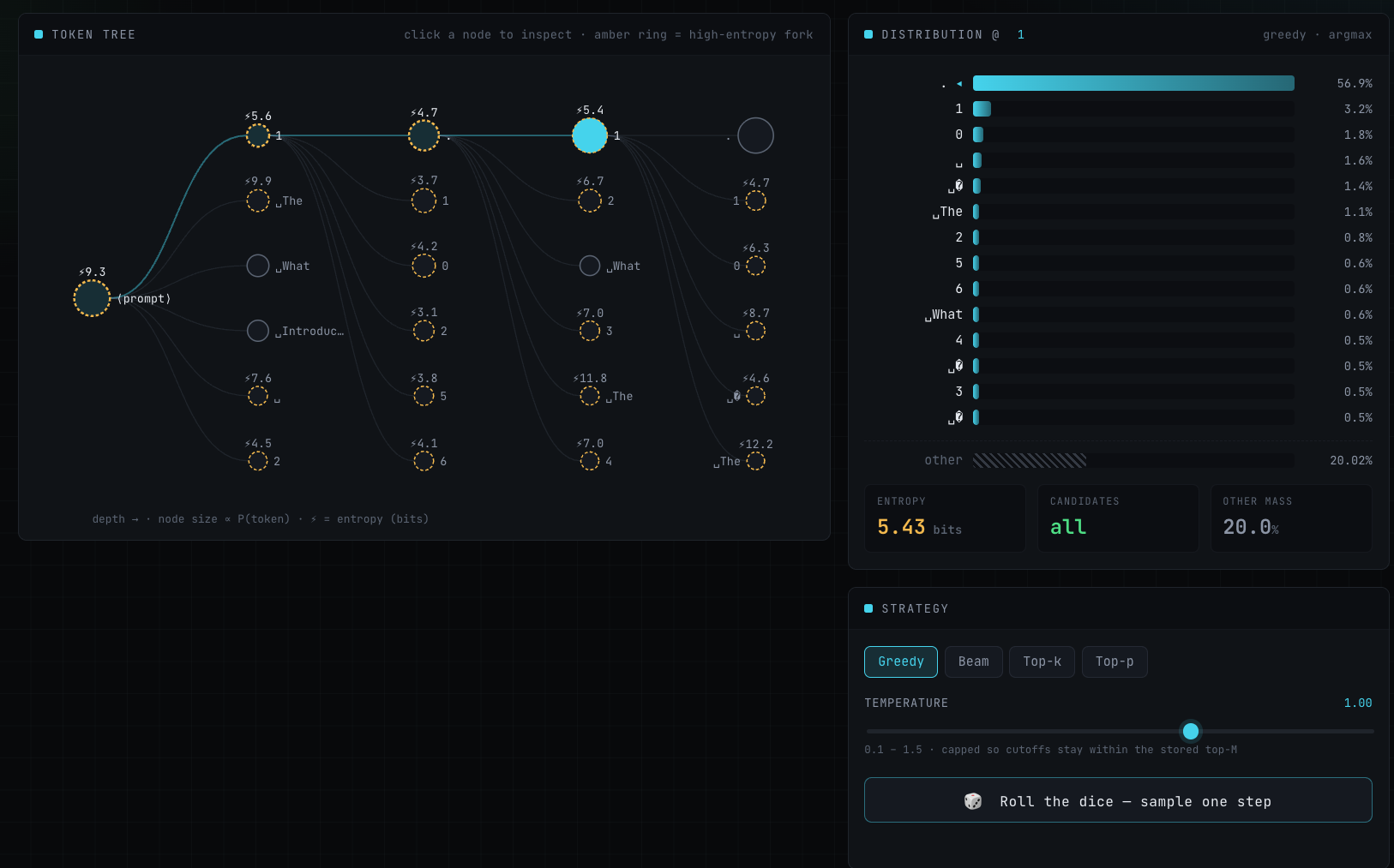
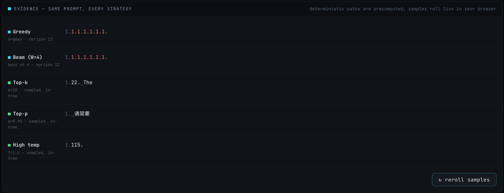
   This is perhaps the most basic one, given the prompt ids, the model does a forward pass, gets the logits of the vocabulary, turns them into a probability distribution via softmax, and picks the token with the highest probability.
   simple, right? But it comes with its consequences…!

2. Beam Search:
   This one was particularly interesting to implement and learn about. Greedy only ever takes the argmax at each step, so it can miss a token that looks worse right now but leads to a higher-probability sequence overall. Beam search fixes this by keeping several candidate paths alive at once, each tracked with its running (cumulative log-) probability. It expands all of them step by step, prunes back to the best few each time, and at the end returns the highest-scoring sequence. Its two knobs are the beam width (how many paths to keep) and the horizon (how many tokens to generate).
   How I implemented it:

def beam_search(model: Model, prompt_ids: Context, width: int, horizon: int) -> list[Hypothesis]:
    """Beam search to `horizon` tokens. Each step expands every live hypothesis by its top-`width`
    candidates, pools them all, and keeps the global top-`width` by cumulative log-prob.
    Returns the W final hypotheses, each (token_ids, cumulative_logprob)."""

    beam = [([], 0.0)]
    for _ in range(horizon):
        candidates = []

        for seq, score in beam:
            logits = next_token_logits(model, prompt_ids+seq)
            log_probs = logits - full_logsumexp(logits)


            for tok, logp in top_m(log_probs, width):
                candidates.append((seq + [tok], score + logp))


        beam = sorted(candidates, key=lambda x:x[1], reverse=True)[:width]
    
    return beam

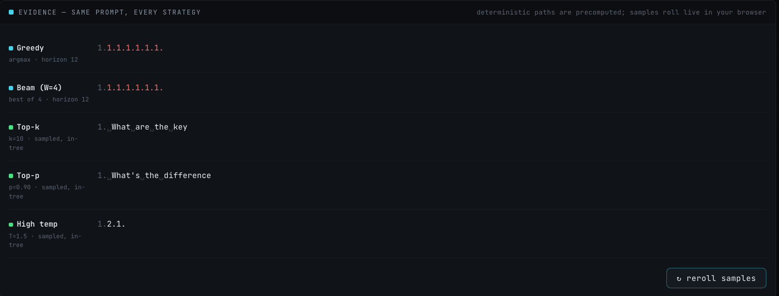
Beam search keeps several hypotheses alive and picks the highest-probability sequence, not just the best next token, so on a normal prompt it can beat greedy. 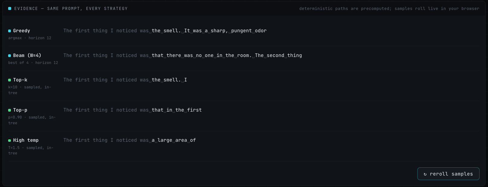But point it at our degenerate 1. and it loops just like greedy because it’s still maximizing probability, and repetition is exactly what high probability looks like.

3. top-k sampling:
   Now, for the heroes of the show. First up, top-k.

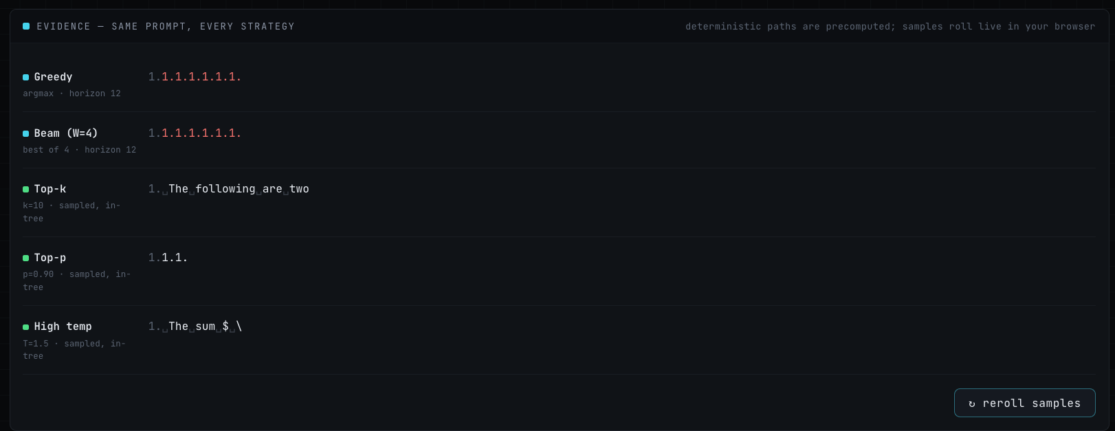
What it does: keep only the k highest-probability tokens, zero out everything else, renormalize over the survivors, and sample one. With k=10, the top 10 tokens (green) survive and the rest are cut: Here k=10 keeps 37% of the mass and discards the rest. And it’s that sample, the bit of randomness greedy and beam never had, that lets it escape the 1. repetition loop you saw in the evidence panel above.

But a fixed k is blunt. Look at where the cutoff lands: it slices straight through a band of near-equal-probability tokens. The last token kept and the first token dropped differ by a hair, decided purely by rank. On a flat distribution like this, k is too restrictive, and the boundary is essentially arbitrary.

Now point top-k at a confident distribution instead, like a deep node in the na na na loop, where the model is ~95% sure the next token is na: Same k=10, but now it’s too permissive: it keeps na (95%) plus nine more tokens that are all under 1%, basically noise it could sample by accident.

Same k, two opposite failures. A fixed rank can’t adapt, because it never looks at the actual probabilities, only their order. That’s the gap top-p closes.

4. top-p (nucleus) sampling:
   Instead of “keep the top k”, top-p keeps the smallest set of tokens whose probabilities sum to p (the nucleus) and samples from those. The cutoff is no longer a fixed count; it grows and shrinks with the model’s confidence.

Take the same confident na node where top-k wastefully kept 10. At p=0.90, the nucleus is a single token: na alone already covers 90%, so nothing else makes it in: Where top-k kept 10, top-p keeps just the one that matters.

Now the opposite: an uncertain step, deep inside a real sentence (“The first thing I noticed was the smell**.**”), where the model has many plausible continuations. The same p=0.90 widens the nucleus to 23 tokens to cover that spread:

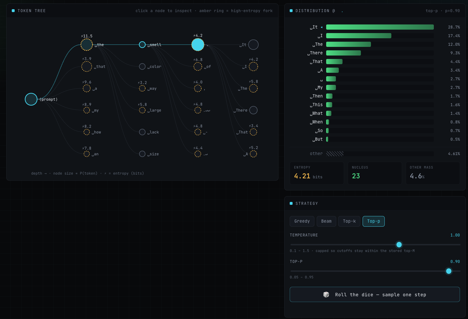
Same p=0.90 both times, and the nucleus went from 1 token to 23 on its own, tracking exactly how sure the model was. That’s the whole point: top-p tightens when the model is confident (so it won’t accidentally sample junk) and loosens when it isn’t (so it stays diverse). That’s the adaptivity a fixed k can never give you.

In conclusion, I really enjoyed learning these strategies via implmentation, and hopefully this blog helped you a little bit as well.
Resources that I used and were a great help, and maybe you should read as well for a good mathematical intuition:\

• “How to generate” by Patrick von Platen
• “The Curious Case of Neural Text Degeneration” by A. Holtzman.

You can find my implementation and vizualizer here:\

• live
• github

Seeya in the next one ;)